How to use Arauto
Arauto was built to be as intuitive as possible. It offers an interface that simulates the line of thinking of analysing and training a model for forecasting. This tutorial will guide you through all the process, starting by the top menus.
Your data menu
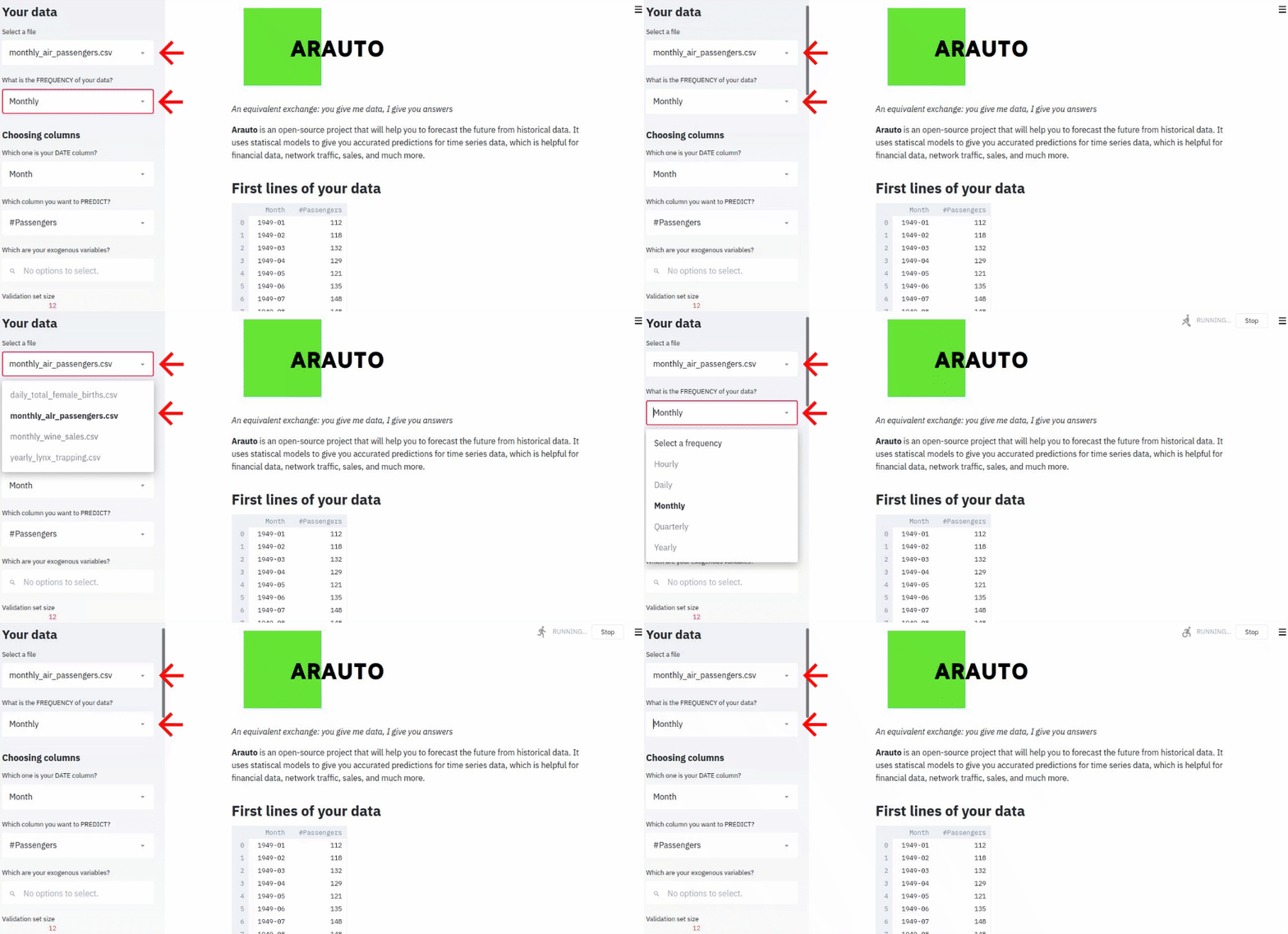
This is where you will pick a file for Arauto to analyse and model. You can play with some toy datasets or you can upload your own dataset using the REST API. You will also select the frequency of your data. If your data was collected in a daily basis, select Daily, if it was collected in a monthly basis, select Monthly. This is an important step since Arauto will use this field to understand the seasonality of the time series, and apply different techniques to find the best model.
Fields
- Select a file: an CSV, TXT, Excel, or delimited file.
- What is the FREQUENCY of your data?: the frequency that the dataset was collected. Null values will be replaced by 0.
Choosing columns menu
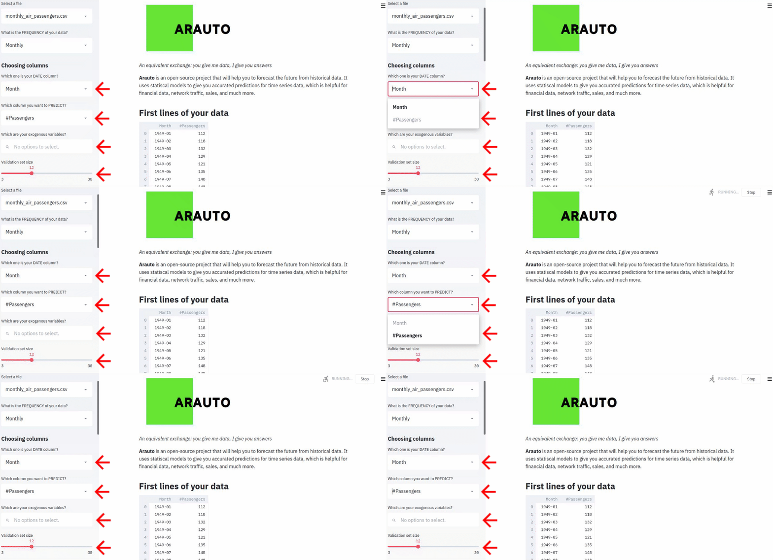
This is step is composed by 4 fields that will instruct Arauto which columns to use when training the model. In this step you can select exogenous variables, what are nothing but columns that will help the model to give different ways for your predictions. For example:
| My Daily Sales | ||
|---|---|---|
| Date | Sales | is_christmas_period |
| 2019-11-29 | 500 | 0 |
| 2019-11-30 | 470 | 0 |
| 2019-12-01 | 200 | 1 |
| 2019-12-02 | 150 | 1 |
Let’s say that you are predicting your company’s daily sales, and in the Christmas period the sales go down. You can use a column called is_christmas_period, where you place 1 for rows (days) on your dataset that was collected in christmas period. Arauto will try to use columns like this to enhance the predictions.
Fields
- Which one is your DATE column?: the column used to identify the time point where the data was collected.
- Which column you want to PREDICT?: the column with the values that you are trying to predict. It can be data like total sales, temperature measured, stock prices, and so on.
- Which are your exogenous variables?: the independent variables (e.g.:
is_christmas_period) that might be important to give different weights to predictions. By informing exogenous variables will use automatically models that support regressors, e.g. ARIMAX. - Validation set size: how many period you want to let for Arauto validate the model? It’s recommended to configure this field with the same amount of periods that you want to forecast. For example, if your data was collected in a monthly basis, and you want to forecast the next 3 months, let this field with value 3.
Charts menu
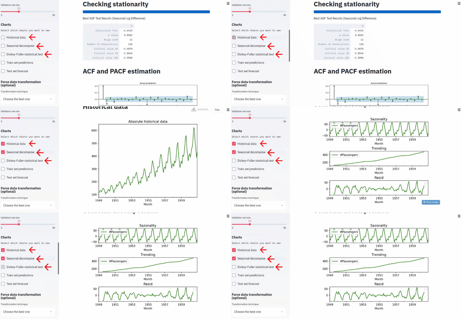
In this section you can select some charts to appear on the screen. These charts are helpful to understand some steps of the model training, like the distribution data, seasonal decompose and out-of-sample predictions.
Fields
- Historical data: show the absolute distribution of your dataset just like it is. It can be useful to understand your data over time, and identify some interesting points like missing values of unusual scales.
- Seasonal decompose: show the components of your time series. It returns informations like the time series trending, seasonality, and resid (what remains when you remove trending and seasonality).
- Dickey-Fuller statistical test: to understand if your time series is stationary (one of the properties that make it possible to forecast data), Arauto will execute the Augmented Dickey-Fuller test (a.k.a ADF test). By enabling this option, the transformed data with the best ADF test result (based on the lowest statistical result) will be plotted on Arauto, with its moving average and standard deviation.
- Train set predictions: enable this option if you wanna check how your model is predicting the data that it was trained with. Two plots are placed in the figure, one for the observed (real) data (labeled as
y), and the predicted data (labeled asŷ). - Test set predictions: enable this option if you wanna check the out-of-sample predictions of your model in comparison with unseen data (test set). Two plots are placed in the figure, one for the observed (real) data (labeled as
y), and the predicted data (labeled asŷ).
Force data transformation menu
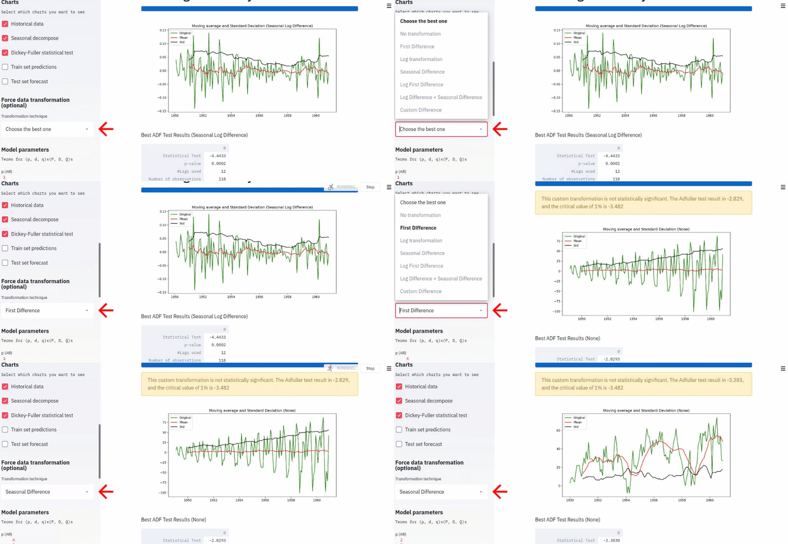
For non-stationary time series (that is, for series that doesn’t have a constant trend and variance over time), Arauto will find the best transformation technique that will make it stationary, hence, making it possible to model and predict the data. By default, Arauto will iterate over all the transformation techniques in order to find the best one, but you can force it to used one of your favorite transformations.
Using the dropdown menu, you can even select to not use any transformation technique on your data. After that, Arauto will execute the Augmented Dickey-Fuller test to check for stationarity. If the test statistics are not significant, Arauto will show a warning. You can continue the process of modeling a time series even with a non-relevant statistical test result, but the model performance might be badly influenced if you select a weak transformation.
Fields There’s just one field on this menu, that is the Transformation technique, which contains the following functions:
Choose the best one: this is the default parameter. Arauto will iterate over all the transformation techniques and select the best one, based on the lowest statistical relevant Augmented Dickey-Fuller test result.
No transformation: No one transformation will be applied on the time series. The ADF test will be executed on the absolute series, without transformations.
First Difference: a First Difference will be applied to the time series. This transformation is made by substraction the current observation from the previou observation. For instance, if you have a series collected in a daily basis, the First Difference of today is equal to: (today_value - yesterday_value). Most of the time series data uses this techniques, which make it stationary. Arauto will always execute this technique first.
Log Transformation: each observation of the series will be log transformed. This is useful when we need to penalize higher values on the time series (which is common when we have outliers in our data). The data is transformed using Numpy’s Log1p function.
Seasonal Difference: if your data contains seasonality, a seasonal difference will be applied on your series. It works similar to First Difference, but instead of substracting the current observation (t) by the previous observation (t-1), Arauto will substract it by the (t-s), where s is the seasonal frequency. For instance, if your data was collected in a monthly basis, and it has a yearly seasonality, the Seasonal Difference will be: (t - t-12).
Log First Difference: this is the first combined transformation that you will see in the dropdown menu. If selected, Arauto will transform your data using Numpy’s Log1p function and, after that, will execute a First Difference transformation (t - t-1).
Log Difference + Seasonal Difference: similar to Log First Difference, Arauto will execute a log transformation in your time series, followed by a First Difference transformation (t - t-1) and a Seasonal Difference (t - t-s), where s is the seasonal frequency.
Custom Difference: you can even select a custom difference technique for your data. This option will enable two other parameters:
Difference sizeandSeasonal Difference size.IMPORTANT: it’s NOT recommended to use more than 1 Seasonal Difference, or more than 2 Differences combined. In other words, your total difference should not pass 2 (seasonal + non-seasonal).
Model parameters menu
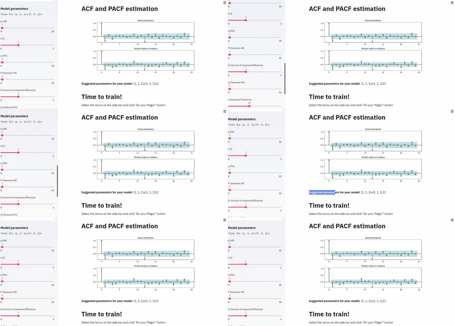
To estimate the right amount of terms to consider for fitting the model, Arauto will look to the ACF and PACF functions to estimate the terms for AR (p), I (d), MA (q), Seasonal AR (P), Seasonal Difference (D), Seasonal MA (Q). By default, Arauto will set a recommended amount of terms for each part, but you can freely select different amounts of terms. Please, refer to How to choose the parameters for the model in order to learn how to select these parameters.
Forecast periods menu
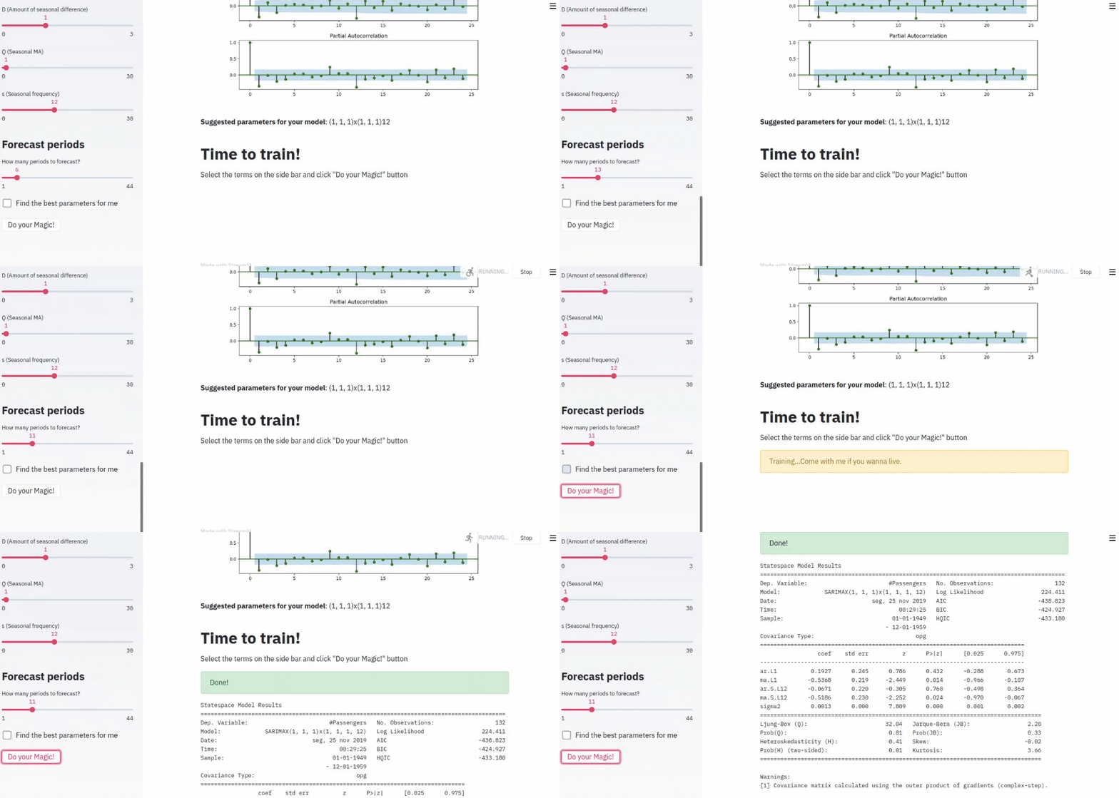
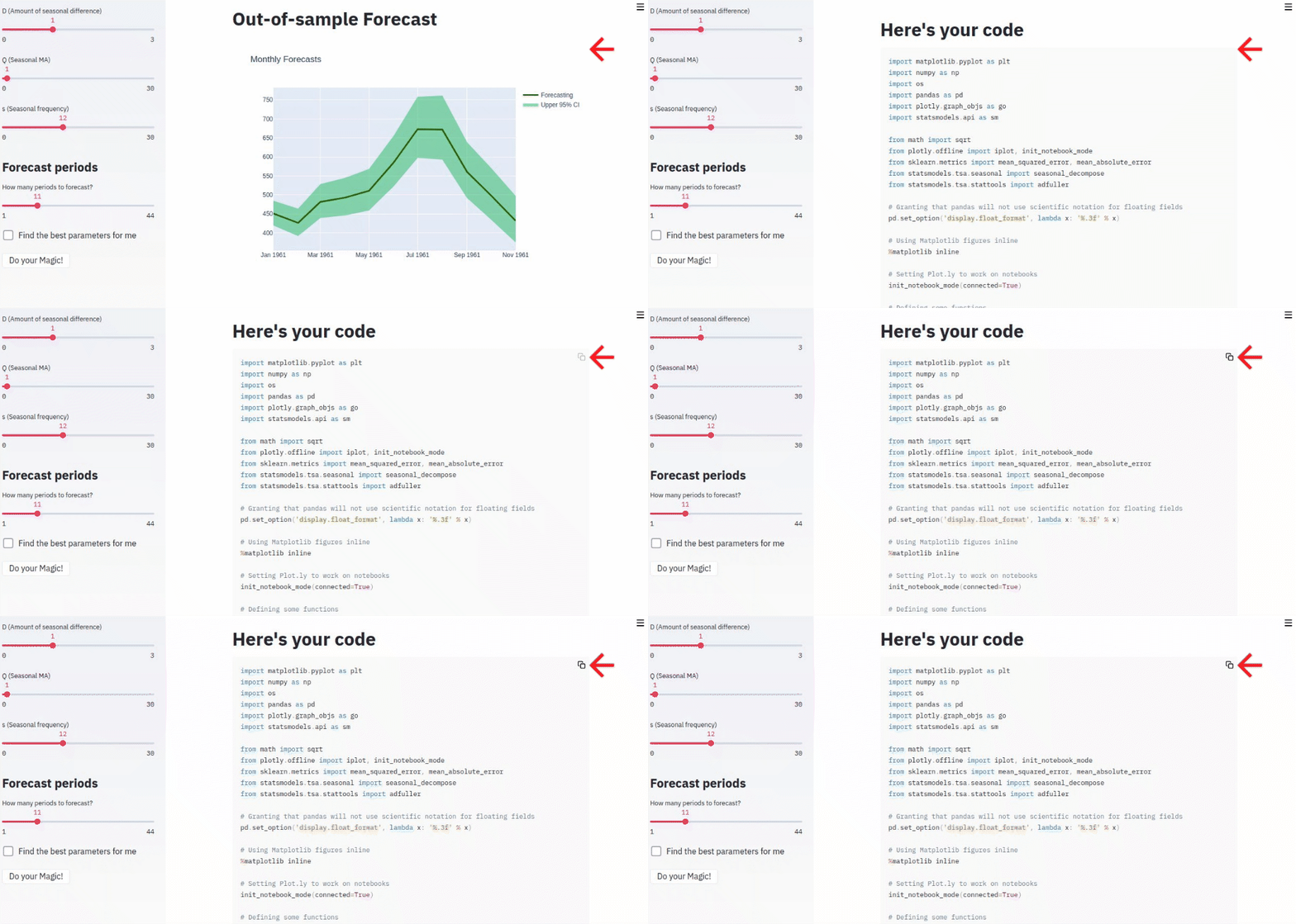
This is the last step of Arauto. Here, you can select how much future periods (days, months, years) you want to forecast.
Fields
- How many periods to forecast?: how much period should Arauto forecast?
- Find the best parameters for me: if selected, Arauto will execute a grid search process to find the best amount of terms for, p, d, q, and so on. This is a high computational process, since Arauto will iterate of different amounts of parameters to fit the best model. Be sure your server has enough memory for this process.
- Do your Magic!: once you have all set up, click this button to train your model.
What happens next?
Once your model was trained, you can check your forecast at the end of you screen. The out-of-sample forecasts are displayed on the screen using Plotly, you can interate with the chart and export it as a PNG image.
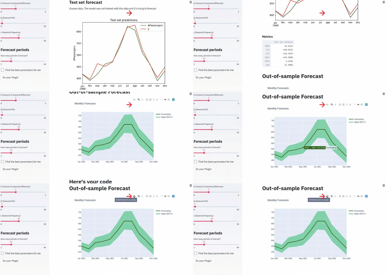
Besides that, Arauto will give the code used to transform the data, generate the charts, train the model, and execute the forecasting. You can copy this code and use it wherever you want.
